Transformations (Part 3)

The first lesson on transformations introduced scaling and translation transformations; the second lesson showed how transformations can be represented using $4 \times 4$ matrices, and also introduced the idea of a composite transformation, formed by multiplying the matrices representing two or more transformations together. Here we’ll add rotation transformations, for rotating about the $x$, $y$ and $z$ axes. In the next lesson we’ll add a transformation that distorts the scene in a way that simulates a 3D perspective effect.

Rotations

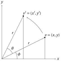
First, rotation about the $z$ axis. Figure 6.1 shows a diagram representing a $z$ axis rotation from vertex $v$ to vertex $v’$. We can represent the coordinates of $v$ in terms of $r$ and $\phi$…

$\begin{aligned} x &= r \cos \phi \\ y &= r \sin \phi \end{aligned}$

…and the coordinates of $v’$ in terms of $r$, $\theta$ and $\phi$:

$\begin{aligned} x' &= r \cos (\phi + \theta) \\ y' &= r \sin (\phi + \theta) \end{aligned}$

We can then use the following identities…

$\begin{aligned} \cos (\phi + \theta) &= \cos \phi \cos \theta - \sin \phi \sin \theta \\ \sin (\phi + \theta) &= \cos \phi \sin \theta + \sin \phi \cos \theta \end{aligned}$

…to rewrite the coordinates of $v’$:

$\begin{aligned} x' = r \cos (\phi + \theta) = r \cos \phi \cos \theta - r \sin \phi \sin \theta \\ y' = r \sin (\phi + \theta) = r \cos \phi \sin \theta + r \sin \phi \cos \theta \end{aligned}$

Substituting $x$ for $r \cos \phi$ and $y$ for $r \sin \phi$, we can get rid of $r$ and $\phi$, so that we have the coordinates of the rotated point $v’$ in terms of only the coordinates of the original point $v$ and the angle of rotation $\theta$:

$\begin{aligned} x' = x \cos \theta - y \sin \theta \\ y' = x \sin \theta + y \cos \theta \end{aligned}$

This is our $z$ axis rotation transformation. It can be rewritten as a matrix multiplication, with the vertices given in homogeneous coordinates:

$\begin{bmatrix} x' \\ y' \\ z' \\ 1 \end{bmatrix} = \begin{bmatrix} x \cos \theta - y \sin \theta \\ x \sin \theta + y \cos \theta \\ z \\ 1 \end{bmatrix} = \begin{bmatrix} \cos \theta & - \sin \theta & 0 & 0 \\ \sin \theta & \cos \theta & 0 & 0 \\ 0 & 0 & 1 & 0 \\ 0 & 0 & 0 & 1 \end{bmatrix} \begin{bmatrix} x \\ y \\ z \\ 1 \end{bmatrix}$

Notice that this transformation makes use of two terms that were zero for the scale and translation transformations, what we might call the “add scaled $y$ to $x$” term (which is set to $- \sin \theta$) and the “add scaled $x$ to $y$” term ($\sin \theta$).

A Yellow Star

Let’s add a $z$ axis rotation function to the scaling and translation functions you wrote for the previous lesson. Add this to the Transform constructor as a public method. (Notice the pb in front of rotateZ.)

// a - Rotation angle in degrees.
//
// Start with current transformation, add a counter-clockwise
// rotation about the z axis.
pb.rotateZ = function (a) {
    var r, s, c;

    r = Math.PI * a / 180.0;
    s = Math.sin(r);
    c = Math.cos(r);

    pv.multiplyBy([ c,   -s,   0.0, 0.0,
                    s,    c,   0.0, 0.0,
                    0.0,  0.0, 1.0, 0.0,
                    0.0,  0.0, 0.0, 1.0 ]);
};

In the same file, we’ll update drawFromBuffer so that it knows about the LINE_LOOP mode:

if (modeString === "LINE_LOOP") {
    mode = pv.gl.LINE_LOOP;
} else if (modeString === "TRIANGLE_FAN") {
    mode = pv.gl.TRIANGLE_FAN;
}

Now we can draw filled or empty squares. Figure 6.2 shows the image generated by the code below. (The order of the vertices is different from examples in previous lessons, which used TRIANGLE_STRIP mode when drawing the square.)

/*jslint white: true */
/*global Canvas, Transform */

(function (global) {
    "use strict";
    var BLACK  = [0.0, 0.0, 0.0],
        YELLOW = [1.0, 0.9, 0.0],
        ORANGE = [0.8, 0.4, 0.0],
        cv, main;

    global.onload = function () {
        cv = new Canvas("canvas", BLACK);
        cv.setupShaders("star.vert", "star.frag",
                "transform", "position", "color", main);
    };

    main = function () {
        var tf, buffer, a;

        tf = new Transform();
        tf.scale(0.75, 1, 1);

        buffer = cv.copyVertexDataToBuffer([
                -0.5,  0.5,  0.0,
                -0.5, -0.5,  0.0,
                 0.5, -0.5,  0.0,
                 0.5,  0.5,  0.0 ]);

        cv.clear();

        for (a = 0; a < 360; a += 36) {
            tf.rotateZ(36);

            tf.scale(0.5, 0.5, 0.5);  // Half size.
            cv.setTransform(tf);
            cv.setColor(YELLOW);
            cv.drawFromBuffer(buffer, 0, 4, "TRIANGLE_FAN");
            tf.scale(2.0, 2.0, 2.0);  // Back to normal size.

            cv.setTransform(tf);
            cv.setColor(ORANGE);
            cv.drawFromBuffer(buffer, 0, 4, "LINE_LOOP");
        }
    };
}(this));

A Different Yellow Star

In the previous example, the coordinate system was rotated about the $z$ axis, $x = y = 0$. What if we wanted to rotate around a different axis, say, $x = y = \frac{1}{2}$? We can do it by creating a composite transformation:

Translate so that $(0.5, 0.5)$ is moved to where the origin was. (That is, translate by $-0.5$ in the $x$ and $y$ directions.)
Then rotate around the $z$ axis, which goes through the new origin.
Then translate back, so that the origin is where it was originally.

The code below shows these three transformations, used to rotate around the axis $x = y = \frac{1}{2}$ (with a rotation angle different from that of the previous example, to make a different kind of star shape).

for (a = 0; a < 360; a += 45) {

    // Rotate around the axis x = y = 0.5.  This is
    // accomplished by 1) translating so that the desired
    // axis of rotation is now the z axis, 2) rotating, and
    // 3) translating back, so that it's as if the whole
    // coordinate system had only been rotated.
    tf.translate(-0.5, -0.5, 0.0);
    tf.rotateZ(45);
    tf.translate(0.5, 0.5, 0.0);

    tf.scale(0.5, 0.5, 0.5);
    cv.setTransform(tf);
    cv.setColor(YELLOW);
    cv.drawFromBuffer(buffer, 0, 4, "TRIANGLE_FAN");
    tf.scale(2.0, 2.0, 2.0);

    cv.setTransform(tf);
    cv.setColor(ORANGE);
    cv.drawFromBuffer(buffer, 0, 4, "LINE_LOOP");
}

The image produced by this code is larger, and is not centered at the origin. To get what you see in figure 6.3, you also need to change the transformation you start with, before you get to the loop:

tf = transform();
tf.scale(0.375, 0.5, 0.5);   // Fix aspect ratio, but also make
                             // everything smaller.
tf.translate(0.5, 0.5, 0.0); // Move origin so that image will
                             // be centered.

A (Slightly) Different Different Yellow Star

If you look closely at figure 6.3, you’ll see that it seems to have a small mistake. The “northeast” yellow square does not have an orange line through it. This is because of the order the filled and unfilled squares were drawn. Remember, whatever is drawn sooner will be covered by what is drawn later. The unfilled orange square whose line would have gone through that yellow square must have been drawn before the square was.

How can we fix this? There are two ways. First, you could make it so that all of the filled yellow squares are drawn before all of the unfilled orange ones—you could use two separate loops. But there’s another way to fix this problem, one that will introduce a new and very important feature of WebGL: the depth test.

Recall that, when you clear the canvas, you pass the argument gl.COLOR_BUFFER_BIT to gl.clear. That is, you clear the color buffer. This is a buffer that stores the color of every pixel in the canvas. Another buffer, the depth buffer is used to store a value representing the depth of each pixel in the canvas. But wait, what is the depth of a pixel? That doesn’t really make sense. The depth stored for each pixel is actually a number representing the distance from the viewer for the fragment most recently drawn at that pixel. When you turn on the depth test, you are telling WebGL to check, each time a fragment is about to be drawn, that it’s in front of whatever was drawn before at that pixel. If it’s in front, it’s drawn. If not it’s discarded.

To turn on the depth test, add the following statement to the library JavaScript file, just after getting the canvas element’s WebGL context and assigning it to gl:

pv.gl = document.getElementById(id).getContext(
        "experimental-webgl");
pv.gl.enable(pv.gl.DEPTH_TEST);

Also, when you clear the canvas, you need to clear the depth buffer in addition to the color buffer. To clear the depth buffer means to set the depth value associated with every pixel to the far plane forming the back of the canonical view volume. This means that the first fragment drawn at any pixel position will always pass the depth test. Here’s a new version of clear that clears the depth buffer. (Together with this change you’ll also want to add bitwise: true to the /*jslint comment line at the beginning, since JSLint assumes by default that | should be ||.)

pb.clear = function () {
    pv.gl.clear(
            pv.gl.COLOR_BUFFER_BIT | pv.gl.DEPTH_BUFFER_BIT);
};

And here’s a new version of the loop from the previous example, modified to put all the unfilled orange squares in the front (without using two separate loops). Figure 6.4 shows the image produced by this version of the program.

for (a = 0; a < 360; a += 45) {
    tf.translate(-0.5, -0.5, 0.0);
    tf.rotateZ(45);
    tf.translate(0.5, 0.5, 0.0);

    tf.translate(0.0, 0.0, 0.1);   // Move back.

    tf.scale(0.5, 0.5, 0.5);
    cv.setTransform(tf);
    cv.setColor(YELLOW);
    cv.drawFromBuffer(buffer, 0, 4, "TRIANGLE_FAN");
    tf.scale(2.0, 2.0, 2.0);

    tf.translate(0.0, 0.0, -0.1);  // Move forward.

    cv.setTransform(tf);
    cv.setColor(ORANGE);
    cv.drawFromBuffer(buffer, 0, 4, "LINE_LOOP");
}

**Figure** : A (Slightly) Different Different Yellow Star

A Purple Cube

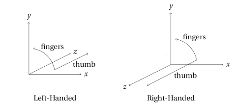
Notice that, in the previous example, to move back meant translating in the positive $z$ direction; to move forward meant translating in the negative $z$ direction. This is because the coordinate system of the canonical view volume is left-handed. That is, if you point the fingers of your left hand from the positive end of the $x$ axis to the positive end of the $y$ axis, your thumb ends up pointing in the direction of positive $z$. Figure 6.5 is meant to illustrate this and to contrast it with a right-handed version of the same idea.

**Figure** : Left- and Right-Handed Coordinate Systems

The canonical view volume coordinate system is left-handed. But a right-handed coordinate system is what you are probably used to using. And just one small change in the code makes it possible to use a right-handed coordinate system when specifying the location of vertices. When we create the initial transform, the one that corrects the aspect ratio, centers and adjusts the size of the image, we negate the $z$ value in the scaling transformation:

tf = transform();
tf.scale(0.375, 0.5, -0.5);   // Negative z, if x and y are
                              // positive, changes the "handedness"
                              // of the coordinate system.
tf.translate(0.5, 0.5, 0.0);

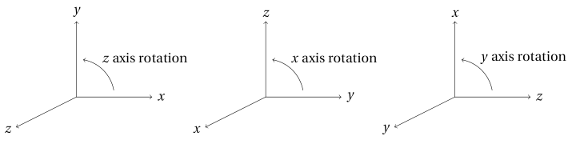
Now that we know the “handedness” of our coordinate system (it’s right-handed), we can picture it in different orientations, as shown in figure 6.6. What’s the point of this? It shows that…

An $x$ axis rotation is like a $z$ axis rotation; just substitute $y$ for $x$, $z$ for $y$, and $x$ for $z$.
A $y$ axis rotation is like a $z$ axis rotation; just substitute $z$ for $x$, $x$ for $y$, and $y$ for $z$.

Here are our $z$ axis equations. ($z’$ = $z$ was excluded before, until we moved to the matrix representation.)

$\begin{aligned} x' &= x \cos \theta - y \sin \theta \\ y' &= x \sin \theta + y \cos \theta \\ z' &= z \end{aligned}$

Substituting $y$ for $x$, $z$ for $y$, and $x$ for $z$, we get equations for an $x$ axis rotation:

$\begin{aligned} y' &= y \cos \theta - z \sin \theta \\ z' &= y \sin \theta + z \cos \theta \\ x' &= x \end{aligned}$

Here’s the (equivalent) $x$ axis rotation written as a matrix multiplication, with the vertices given in homogeneous coordinates.

$\begin{bmatrix} x' \\ y' \\ z' \\ 1 \end{bmatrix} = \begin{bmatrix} x \\ y \cos \theta - z \sin \theta \\ y \sin \theta + z \cos \theta \\ 1 \end{bmatrix} = \begin{bmatrix} 1 & 0 & 0 & 0 \\ 0 & \cos \theta & - \sin \theta & 0 \\ 0 & \sin \theta & \cos \theta & 0 \\ 0 & 0 & 0 & 1 \end{bmatrix} \begin{bmatrix} x \\ y \\ z \\ 1 \end{bmatrix}$

Or, if we go back to the $z$ axis rotation equations and substitute $z$ for $x$, $x$ for $y$, and $y$ for $z$, we get equations for a $y$ axis rotation:

$\begin{aligned} z' &= z \cos \theta - x \sin \theta \\ x' &= z \sin \theta + x \cos \theta \\ y' &= y \end{aligned}$

Here’s the $y$ axis rotation written as a matrix multiplication:

$\begin{bmatrix} x' \\ y' \\ z' \\ 1 \end{bmatrix} = \begin{bmatrix} z \sin \theta + x \cos \theta \\ y \\ z \cos \theta - x \sin \theta \\ 1 \end{bmatrix} = \begin{bmatrix} \cos \theta & 0 & \sin \theta & 0 \\ 0 & 1 & 0 & 0 \\ - \sin \theta & 0 & \cos \theta & 0 \\ 0 & 0 & 0 & 1 \end{bmatrix} \begin{bmatrix} x \\ y \\ z \\ 1 \end{bmatrix}$

Once you’ve added rotateX and rotateY functions to the library file and completed the code below (exercise 6.1), you should get what you see in figure 6.7.

/*jslint white: true */
/*global Canvas, Transform */

(function (global) {
    "use strict";
    var BLACK  = [0.0, 0.0, 0.0],
        PURPLE = [0.7, 0.0, 1.0],
        cv, main;

    global.onload = function () {
        cv = new Canvas("canvas", BLACK);
        cv.setupShaders("cube.vert", "cube.frag",
                "transform", "position", "color", main);
    };

    main = function () {
        var tf, buffer, draw;

        tf = new Transform();
        tf.scale(0.6, 0.8, -0.8);  // Fix aspect ratio, make things
                                   // a little smaller.

        tf.rotateX(30);            // Tilt the view point up.
        tf.rotateY(-15);           // Turn things a little to the
                                   // left.

        tf.translate(-0.6, -0.8, 0.0);  // Center things in canvas.

        buffer = cv.copyVertexDataToBuffer([
                0.0,  1.0,  0.0,
                0.0,  0.0,  0.0,
                1.0,  0.0,  0.0,
                1.0,  1.0,  0.0 ]);

        cv.clear();

        draw = function () {
            cv.setTransform(tf);
            cv.setColor(PURPLE);
            cv.drawFromBuffer(buffer, 0, 4, "TRIANGLE_FAN");
            cv.setColor(0.0, 0.0, 0.0);
            cv.drawFromBuffer(buffer, 0, 4, "LINE_LOOP");
        };

        // Draw front of cube.
        draw();

        // Draw right side.
        tf.rotateY(90);
        tf.translate(0.0, 0.0, 1.0);
        draw();

        // Exercise 1...
    };
}(this));

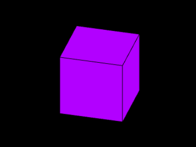
The image shown in figure 6.7 is your very first 3D thing! (Once you’ve completed exercise 6.1.) But it looks a little strange, almost as if the back of the cube is slightly bigger than the front. It isn’t actually bigger, it’s the same size. But we’re used to farther away things looking smaller than closer things, so when they’re the same size the farther thing looks like it must be bigger. We’ll see in the next lesson how to fix this.

Exercise : Add rotateX and rotateY functions to the library file, following the pattern of rotateZ above. Then complete the code for the fourth example so that you see the purple cube. Because you can’t see all six sides at once, check your program by commenting out some, then commenting out others, etc.